Holonomy, curvature, and the information carried by loops

Close a path and inspect what remains

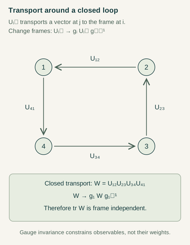
Take an oriented square x₀→x₁→x₂→x₃→x₀. With U_yx:V_x→V_y, the based holonomy is

It compares the initial amplitude with the amplitude transported around the whole loop. Under independent local changes, W′_x₀=g_x₀W_x₀g_x₀⁻¹. The loop matrix is therefore presentation dependent, but its conjugacy class is independent of the base frame. Reversing the loop gives W†, and the eigenangles change sign.

The determinant, traces of powers, and spectrum are conjugation invariant. The expectation ψ†Wψ is also invariant if the probe state is transformed with its base frame. Which of these quantities can be measured depends on the prepared carrier and interference protocol. Holonomy is thus relational data rather than an isolated matrix with a preferred basis. Theorem 5.2 and Proposition 5.3, pp.10–11.

A loop can be a sequence of internal comparisons, not necessarily a particle’s spacetime orbit. Identifying its geometry with a physical spatial loop requires an operational relation between record adjacency, displacement, and the detector. The temporal interpretation does not supply that relation merely by assigning names to inner generative stages.

Separate removable tree links from independent cycles

Choose a root in a connected finite graph and a spanning tree. Fix the root frame and recursively choose g_y=g_xU_yx⁻¹ along each parent-to-child tree edge. Every transformed tree link is I. Each edge outside the tree closes one fundamental cycle, leaving |E|−|V|+1 independent generators of graph path comparison. This is a graph-theoretic counting statement, not a count of independent scalar observables or physical gauge bosons. Proposition 5.3, p.11.

The remaining loop matrices are all based at the same root and transform by simultaneous conjugation. Their individual spectra can omit information about their relative orientations. For example, two SU(2) loop matrices can be U=iσ_z, V=iσ_z, or U=iσ_z, V=iσ_x. In both configurations each separate loop has eigenvalues +i and −i and trace zero. However, Tr(UV)=−2 in the first and Tr(UV)=0 in the second.

Products and commutators of loops therefore matter on a graph with more than one cycle. The complete comparison record concerns the tuple modulo a common conjugation, with the actual test family determining how much of that tuple must be retained. Discarding all relative orientation data simply because each isolated Wilson trace agrees can destroy predictive sufficiency.

Extract curvature from an area-order response

Use D=d+A with A anti-Hermitian and forward short transport U_x+dx,x=I−A_μdx^μ+⋯. Traverse a small coordinate rectangle in the order +μ,+ν,−μ,−ν. Expanding its four correctly ordered links gives

Here ℓ denotes a common small side scale and the remainder assumes a sufficiently smooth connection. Reversing orientation reverses the leading sign. The derivative terms compare the connection at neighboring points; the commutator records the order dependence of the matrix operations. Curvature is the infinitesimal failure of local path independence.

A nontrivial loop at one finite size is insufficient evidence for a nonzero local curvature. To infer F operationally, one needs a family of shrinking contractible loops, an area normalization, and control of the higher-order error. The field may also be flat but topologically nontrivial. These qualifications are explicit in the source’s path-to-connection discussion. Corollary 2.4, p.5; §13.3, p.45.

Flat connections can retain global information

Consider a complex line over a circle with connection A=iαdθ, where θ has period 2π. There is no curvature two-form on a one-dimensional base, so F=0. Nevertheless, one forward circuit has holonomy exp(−2πiα), which is nontrivial when α is not an integer. Locally one can remove A by a phase choice; that phase choice fails to be single valued around the circle.

This example separates three statements: locally flat transport, trivial holonomy on every loop, and a globally chosen parallel unit tensor. The last implies the second for its line, while the first alone does not. In the determinant-linked carrier, the equation TrF₃+TrF₂=0 says that the total determinant connection is flat. To require detW₃detW₂=1 on every loop, including global flat and torsion loops, the manuscript instead supplies a global parallel tensor in detV₃⊗detV₂. Theorem 6.3 and No-go theorem 6.6, pp.12–13.

Ordinary homotopy class can organize flat transport on a suitable base. For a curved connection, contractible loops can carry nontrivial holonomy and their geometry matters. Thin-homotopy invariance in the transport theorem should not be mistaken for invariance under every deformation of a path.

A trace deficit measures unitary mismatch

For any m×m unitary W, its eigenvalues are e^iθa and

It vanishes precisely at W=I. For W=e^iX with a small Hermitian X, the deficit is ½TrX²+O(‖X‖⁴). A square of side a therefore has m−ReTrW=a⁴‖F_μν‖²_HS/2+O(a⁵) in the smooth regime. The leading response is positive and insensitive to reversal of loop orientation.

A specified controlled-loop experiment gives this quantity an operational interpretation. Prepare a maximally mixed carrier I/m, compare W against identity on a coherent two-path control, and measure the minus port. Its probability is (m−ReTrW)/(2m). Choosing an energy penalty of 2mκ per rejection then gives the mean cost κ(m−ReTrW). The experiment and its energy assignment are separate inputs. Propositions 17.3–17.4, p.53.

The smooth lattice expansion establishes a deterministic comparison-cost limit under its assumed dimension and regularity. It does not construct a quantum measure, prove confinement, or establish a continuum mass gap. The effective-interactions guide distinguishes a chosen trace cost from a generated Hamiltonian term.

A determinant-linked central loop is a useful worked example

In the primitive integral central normalization, take W₃=e^−2ifI₃ and W₂=e^3ifI₂. Their determinants are e^−6if and e^6if, so the total determinant is exactly one for every f. The two blocks still have nontrivial relative phase transport.

The numbers 12 and 18 come from rank times squared defining charge: 3×(−2)² and 2×3². They are representation-trace factors in this declared cost model. They are not the number of inner temporal stages, and the coefficient relation does not by itself determine measured coupling constants. The exact independent singlet Hamiltonian has the same quadratic relation with its exact energy Hessian coefficients; it need not have the same full finite-angle potential. Corollary 2.4, p.11; §17.4, p.54.

A forced circuit followed only by singlet return gives |TrW_m/m|²=1 for either central block. The coherent comparison above gives sin²(q_mf/2), with q₃=−2 and q₂=3. The difference is in the experiment, not in whether the holonomy exists.

Protected carriers need not be geometrically flat

A smooth retained projector P can carry the connection ∇=Pd and curvature P(dP∧dP)P. To see that a fixed gap does not force flatness, supply a graph embedding u_Z=(I,Z)^T(I+Z†Z)^−1/2, let P_Z=u_Zu_Z†, and choose H_Z=δ(I−P_Z) with δ>0. The rank-m zero-energy cluster stays separated by exactly δ as Z varies.

At a point with Z=0 the curvature is dZ†∧dZ. For Z(x,y)=xI+yB and B†=−B, F_xy(0)=2B. Every anti-Hermitian matrix direction is thus available in this supplied embedding family. For paired blocks, the determinant condition requires the corresponding total-trace correction. Proposition 14.1 and Theorem 15.2, pp.45–47.

This is an existence and local-accessibility calculation. It assumes the open-completion embedding modes and their permitted controls. Varying only the bare oriented quaternionic source frame in the stipulated seven-clock construction leaves the relevant projectors geometrically flat. The allowed frame group, the source’s actual variations, and the realized holonomy group must therefore be distinguished.

What a source model must add to loop geometry

Loop geometry answers a precise question: what changes when retained amplitudes are compared along different histories? A model of physical gauge fields must also determine which links fluctuate, their conjugate electric variables, the state space and constraints, the Hamiltonian or action, and the observables used for physical matching. A background Berry connection can produce observable phases without becoming an autonomous propagating gauge field.

The source manuscript’s flat countermodel has constant carrier projectors, identity links, and the same finite source and completion structure as its nonflat candidates. Conversely, the graph-embedding model shows nonzero curvature without changing the protected eigenvalues. Together they rule out identifying source recurrence, spectral gap, curvature, and field dynamics as one quantity. Proposition 9.2, p.18; §§14–15 and §21, pp.45–47 and 63–64.

A useful next test is therefore conditional and quantitative: specify a record family, measure or calculate its transport on shrinking loops, show which reference resources make that signal visible, and derive the response from the proposed dynamics. The exact singlet-response model supplies one tractable finite example of such a calculated loop dependence.

Continue reading

• Ordered transport and the connection
• Which loop information is observable?
• Winding, topology, and charge
• An exact holonomy response