

Assumptions, results and research status
Exact mechanisms; conditional physical application
Assumptions
- A self-adjoint Hamiltonian and a declared retained/auxiliary decomposition are supplied.
- The eliminated block is invertible at the energy under consideration; form-domain conditions replace bounded-block assumptions when necessary.
- A gap estimate is formulated only after the physical vacuum has been removed or transported exactly.
- The six nested inner levels and seventh completion supply an interpretation; they do not independently fix the auxiliary Hamiltonian or its coefficients.
Results
- Schur elimination gives an exact energy-dependent effective operator.
- Virtual excursions and constrained minimization produce explicit interactions with model-dependent coefficients.
- Norm or relative-form error estimates determine the regime in which an effective law predicts dynamics.
Open questions
- Can one completion rule select the auxiliary gap, hopping, kinetic normalization and retained carrier together?
- Can the auxiliary completion band be eliminated uniformly in physical volume and regulator resolution?
- Do the induced interactions converge to the required four-dimensional gauge theory?
What an effective interaction remembers
A retained description records only some variables of a larger system. The omitted variables may be expensive to excite, too fast to resolve, or constrained by the preparation protocol. They still affect the retained variables because an amplitude can enter the omitted sector and return, or because a constraint forces the omitted sector to rearrange. Elimination calculates the resulting change in energy and evolution.
In the SMM/DTT programme, this provides a concrete mechanism by which generative work could affect completed records. It becomes a source derivation only when the same specified completion law determines the carriers, the auxiliary response and the coefficients. A separately selected auxiliary Hamiltonian supplies a valid model calculation, but leaves that common origin as an additional task.
Three operations should be distinguished. Solving the auxiliary equation inside an eigenvalue problem is an exact algebraic reduction. Expanding its inverse in a small parameter is an approximation. Tracing or averaging variables in a state is a different operation and can produce a mixed state with memory. Agreement between these operations requires assumptions about preparation, energy range and time scales.
Source: Vacuum obstructions and form Feshbach reduction, §10, pp.23–25.
Derive the retained operator
Write the Hilbert space as a direct sum of retained and auxiliary sectors, with orthogonal projections P and Q. On a finite model, or under the bounded-block hypotheses stated in the source, the Hamiltonian has blocks A=PHP, B=PHQ and D=QHQ. An eigenvector has components x and y. Its auxiliary equation reads B†x+(D−E)y=0.
Heff(E)=A−B(D−E)−1B†,
[Heff(E)−E]x=0.
This formula is exact when D−E is invertible. It is energy dependent because the response of the omitted sector depends on the frequency of the retained motion. If D≥Γ and E<Γ, the correction is negative semidefinite: mixing with a higher sector lowers the retained energy relative to the uncoupled block A.
If ∥B∥≤b, spectral calculus gives an explicit bound, 0≤B(D−E)−1B†≤b²/(Γ−E). The useful small quantity is therefore the correction compared with the accuracy or spectral margin being sought. A large Γ alone is insufficient if the coupling b increases at the same time.
For a physical mass-gap calculation, first remove the vacuum. If the chosen P divides the vacuum between its two ranges, use the transported-vacuum construction before imposing strict low-sector positivity. The ordinary algebra does not permit the zero-energy state to be assigned a positive excitation energy.
Source: Vacuum obstructions and form Feshbach reduction, §§6 and 10, pp.15–18 and 23–25.
An exact two-state calculation
Take the real symmetric matrix with diagonal entries 0 and Δ>0 and off-diagonal coupling g. Its lower eigenvalue and small-coupling expansion are
=−g²/Δ+g⁴/Δ³+O(g⁶/Δ⁵).
Setting E=0 in the exact eliminated denominator gives the leading shift −g²/Δ. At g=0.1Δ, this approximation is −0.01Δ, whereas the exact answer is about −0.00990195Δ. The discrepancy is about 0.00009805Δ. Both the coupling ratio and the requested absolute accuracy matter.
An elementary exact remainder bound is available without trusting a series. Rationalizing the square root gives E−=−2g²/[Δ+√(Δ²+4g²)]. Consequently 0≤E−+g²/Δ≤g⁴/Δ³. This certifies the leading answer for every real g, although the certificate is informative mainly when |g|/Δ is small.
The omitted amplitude is y=gx/(E−Δ). A low-energy eigenvector is therefore dressed by an auxiliary component. Preparing only its bare retained component changes the initial condition. An effective energy calculation and a preparation calculation answer related but different questions.
The negative lower energy is measured relative to the uncoupled reference. Subtracting the exact ground energy makes the full Hamiltonian nonnegative; it does not erase the energy differences that encode the induced interaction.
Why a virtual loop knows about holonomy
Gauge transport gives each hop a matrix. A virtual excursion that returns to its starting carrier multiplies the transports in path order. Under Uyx↦gyUyxgx−1, all interior frame changes cancel. A closed product transforms by conjugation at its base point, so its trace can enter a gauge-invariant effective energy.
In the supplied four-position singlet model, a complete circuit first contributes at fourth order in hopping. The static small-hopping response, with carrier rank m, binding penalty Δ and hopping t, is
The second-order excursion goes out and back and has no holonomy dependence. The fourth-order circuit can distinguish W. Intermediate returns and the normalization of the energy-dependent reduction must be included; counting only visibly circulating paths can miss cancellations.
The singlet-loop guide derives the finite model and the holonomy-Hessian guide explains its response coefficients. This apparatus selects a loop interaction after its gap and hopping have been supplied. Exact gauge invariance fixes the allowed transformation law, while this dynamics fixes the numerical response within the stated model.
A classical mediator gives a different exact law
There is a parallel mechanism that uses constrained minimization. Let B be the edge-by-vertex incidence matrix of a connected finite graph. Then L=BᵀB is the graph Laplacian, with constants as its kernel. A vertex source ρ is admissible when its total sum is zero. Let G=L+ denote the inverse on the mean-zero subspace.
For η>0, minimize the positive edge-flux energy (η/2)∥F∥² subject to BᵀF=ρ. The candidate F*=BGρ satisfies the constraint because LGρ=ρ. Any other feasible flux is F*+z with Bᵀz=0, and its cross term vanishes:
minBᵀF=ρ(η/2)∥F∥²=(η/2)ρᵀGρ.
The inverse Laplacian makes the interaction nonlocal even though the original flux energy is a sum over edges. On a single edge connecting two vertices, a neutral source (q,−q) fixes a flux of magnitude |q| and costs ηq²/2. On a larger graph, available paths redistribute that flux and change the cost.
Writing ρ as a sum of two source patterns exposes self-energies and a cross term ηρ₁ᵀGρ₂. Its sign depends on the source patterns and the chosen reference for the Green function. This is a quasistatic response calculation; quantized propagating mediator modes require a dynamical model with a kinetic term and a quantum state space.
Convert an operator error into a useful time
Suppose two self-adjoint Hamiltonians on the same finite retained space differ by a bounded operator R with ∥R∥≤r. Duhamel’s identity inserts R once between two unitary evolutions. Taking norms and using unitarity yields
For an evolution error at most ε, the sufficient interval is |t|≤εℏ/r. Here r is an energy, so the ratio is dimensionless. A very small energy correction can accumulate into a significant phase over a long observation time. Conversely, a bound larger than two supplies no useful accuracy information because two unitaries already differ by at most two.
A comparison through a dressing isometry must include that isometry on both sides. If the prepared state differs from the dressed state by εprep, a simple triangle estimate adds the preparation error to the dynamical error. Finite representation compression can create further boundary terms by spoiling exact unitary link identities.
The unbounded lattice setting usually requires relative-form estimates and controlled resolvents instead of a global bounded difference. The finite norm calculation remains a useful benchmark, but its hypotheses must not be silently imported into an infinite-dimensional gauge Hamiltonian.
Source: Vacuum obstructions and form Feshbach reduction, §10, pp.23–25.
Gauge invariance survives compatible elimination
At a finite Euclidean regulator, define an effective weight by integrating the auxiliary variables y at fixed retained configuration U:
If the original action and conditional measure transform equivariantly, changing integration variables by the gauge transformation shows Seff(g·U)=Seff(U). This conclusion is exact and does not need a perturbative expansion. It restricts the operators that may appear after elimination, including closed-loop functions and invariant curvature terms.
The conclusion does not imply that the induced action is short range. That requires decay of connected auxiliary correlations and a bound on the resulting connected interactions. Nor does it determine the plaquette coefficient: a physical renormalization condition is still required.
A bare local closure coefficient tending to zero is also insufficient. There is one closure term per site, and the number of sites grows. The source therefore asks for the induced interactions to vanish in a volume-independent local norm, after connected cumulants and geometric band corrections have been included.
Source: Auxiliary-time lattice gauge framework, §19, printed pp.47–49.
What would make this a stronger source explanation
A useful source-level result would constrain several quantities that the model currently permits one to choose independently. For example, a specified nested completion process might determine an auxiliary gap, a hopping amplitude and a clock response, giving a testable relation between the induced loop coefficient and that clock response. The relation should survive elimination and be consistent across more than one preparation protocol.
The six inner levels should enter as explicit nested dependencies, with the seventh stage completing the retained record. Introducing a cyclic regulator is a declared modelling choice within that research strategy. Its finite Fourier modes are not additional independent temporal axes.
The present calculations establish real mechanisms: block response, virtual holonomy and constrained flux all leave calculable effective interactions. The remaining tasks concern selection and control. Which Hamiltonian follows from the proposed source? Which band is physically retained? Which corrections remain small in large volume? Which observables and units connect the effective coefficient to experiment?
For the auxiliary lattice programme, the immediate analytic milestone is a genuine nonlinear fast band with small derivative and mixing corrections. Even success there leaves the four-dimensional nonabelian infrared problem to be proved separately.
Source: Auxiliary-time lattice gauge framework, §§16.8, 19.4–19.6 and 24.3, printed pp.43,48–49,55.
Continue reading
Sources for this guide
Source manuscripts, version notes, and standard references are listed in the reference library.