Singlet loops: a supplied microscopic Hamiltonian with a generated response

Why this model is useful

The operational reconstruction explains why sufficient records may need relational transport. It does not determine an energy for that transport. The singlet-loop model supplies a separate, fully specified finite Hamiltonian and asks what energy response follows. Its results can be checked without assuming SMM/DTT; the temporal interpretation is a proposed physical use of the construction. §§1–2, pp.5–12.

The model has no bare plaquette trace term. Its microscopic interaction moves a carrier between neighboring positions, while a binding penalty favors return to a root singlet. Virtual circuits then produce a holonomy-dependent energy. This makes the origin of the coefficient and its domain of control visible. It does not establish that the chosen hopping law and penalty are uniquely generated by an ontology.

The site uses m=2 and m=3 for the two retained blocks. The one-block static equation accepts any W∈U(m); a combined determinant-linked configuration additionally satisfies detW₃detW₂=1. Exploring one block independently is a valid diagnostic of the block Hamiltonian and should be labeled accordingly.

Construct the auxiliary space and its root singlet

Label the cycle positions 0,1,2,3. Let V_m,j be a rank-m carrier at position j and let V_m,0* be a dual reference that remains at the root. The auxiliary space is

The root singlet is |s_m〉=m^−1/2Σ_a=1^m|0,a〉⊗|ā〉. It is the normalized identity contraction, so simultaneous carrier and dual basis changes leave it invariant. Set P_m=|s_m〉〈s_m| and Q_m=I−P_m. The root position is selected, but no root color frame is preferred. §2.1, p.8.

The stationary dual is physical comparison data in this model. It must not be described as a reference that local selector noise has already erased. In the joint record instrument, the singlet probe and the protected right records are separate factors. If a proposed Hamiltonian acts directly on the right carriers instead, their pointwise preservation must be checked again.

State every term in the Hamiltonian

For the directed edge j→j+1, define T_j,m to move the carrier with U_j+1,j;m, act as identity on the dual, and vanish on the other position summands. Indices are taken modulo four. Choose

All nonroot positions and all root nonsinglets cost Δ_m. Penalizing position alone would leave additional unpenalized root states and would define a different model. The cycle has degree two, giving ‖V_m‖≤2|t_m| for its hopping part. Elementary perturbation bounds isolate the zero-energy continuation when |t_m|<Δ_m/4; the exact static theorem later removes that restriction for ground-state isolation.

The binding scale Δ is supplied. It is not the seven-clock chord response, the logarithmic source frequency, or the doubled-cut singular gap. Under a frame change, links obey U′_yx=g_yU_yxg_x⁻¹, and the auxiliary at position j transforms as g_j⊗ḡ₀. Both terms transform consistently. §2.1, pp.8–9.

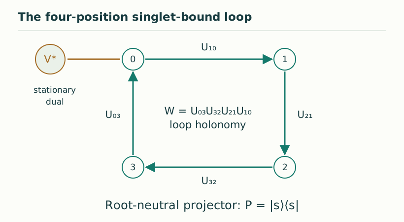
A carrier–dual contraction turns a circuit into a trace

The forward cycle product is W=U_0,3U_3,2U_2,1U_1,0. Transporting the carrier once around it gives the singlet contraction

The opposite orientation gives its complex conjugate. This normalized trace comes from a prepared invariant carrier–dual contraction; it is not inserted afterward by averaging over a chosen color component. A closed virtual loop is therefore a natural place for a gauge-invariant scalar to arise in this Hamiltonian.

At first order, hopping takes the root singlet to a different position and has zero expectation. At second order, the carrier can hop to either neighbor and return immediately; both link products are identity. Odd-order closed hopping paths are absent because the four-cycle is bipartite. The first paths sensitive to full loop holonomy occur at four transfers. These combinatorial facts are tied to the four-position model, not to a universal temporal recurrence count. Theorem 2.5 and its proof, pp.11–12.

Derive the fourth-order energy including the folded term

Suppress the block label, write H=ΔQ+V, and define a₂=〈s|VQV|s〉 and a₄=〈s|VQVQVQV|s〉. Expanding the scalar Feshbach equation while retaining its energy dependence gives

The two unitary backtracks give a₂=2t². In a four-step sequence, an intermediate two-step return to the root is again a singlet and is removed by Q. The allowed remaining paths comprise two retracing excursions through nonroot positions and two oriented full cycles. Thus a₄=t⁴[2+(2/m)ReTrW]. Substitution gives

The positive folded contribution a₂²/Δ³ is essential. Omitting it produces an incorrect holonomy-independent fourth-order energy and spoils the cancellation at W=I. The result is a generated leading trace interaction for this selected Hamiltonian. It is not the claim that its exact finite-hopping potential is a Wilson trace function. Theorem 2.5, pp.11–12.

Use the stated perturbative error and normalization

Let ε=t/Δ. For |ε|<1/4, the source proves a uniform estimate over all unitary W:

The constant is deliberately conservative. It establishes analytic control; it is not an optimized prediction of the numerical error in a particular example. For the normalized response E(W)−E(I), the remainder is R(W)−R(I), so the displayed uniform bound doubles if used directly by the triangle inequality. The exact resolvent is preferable for evaluating a particular finite parameter point. Theorem 2.5, p.11.

The next expansion is E(W)/Δ=−2ε²+2(1−c_W)ε⁴+(12c_W−4)ε⁶+O(ε⁸), where c_W=ReTrW/m. In particular, E(I)/Δ=−2ε²+8ε⁶+O(ε⁸). Subtracting only the second-order constant is therefore not an exact normalization of the potential.

Changing individual positive edge hoppings and nonroot penalties gives the leading coefficient 2Π_j=0³t_j/(mΔ₁Δ₂Δ₃). A positive root-nonsinglet penalty is still required for the starting band. The equal-penalty exact secular equation and its error constant cannot be reused for this modified Hamiltonian without a new derivation.

Use the same singlet as a declared completion outcome

The joint update interprets P as the successful return outcome and ΔQ as its energetic failure penalty. This identification is a proposed microscopic bridge between comparison and completion. Under one uninterrupted coherent interval, define p_W(τ)=|〈s|e^{−iτH(W)/ℏ}|s〉|². With u=τ/ℏ and L=Δ+4|t|, the calculated difference is

The holonomy appears at fourth order because four transfers are needed to distinguish the two circulation orientations from common backtracking histories. The leading Δ-dependent survival terms cancel in this difference. The coefficient is dimensionless and concerns a completion probability; it is not κ^loop or an exact energy stiffness. Theorem 20.4, pp.61–62.

For W=e^iθI, the leading factor is 1−cosθ and is visible. By contrast, forcing exactly one circuit and then checking only the root singlet gives |TrW/m|²=1. Waiting and backtracking amplitudes provide coherent alternatives in the Hamiltonian experiment. Resetting the probe or measuring P/Q repeatedly changes those alternatives and defines another dynamics.

The exact spectral solution extends beyond weak hopping

A spanning-tree frame choice makes three links identity and leaves W on the fourth. Diagonalizing W splits the free carrier motion into twisted four-position rings. The rank-one singlet binding then reduces the ground-state problem to one monotone resolvent equation. For every Δ>0 and real t, the ground state is unique; for m≥2 its exact gap is bounded below by Δ/(4m). The response-and-gap guide derives the equation and a stable numerical solution. Theorem 2.1, pp.9–10.

The exact identity Hessian is E(e^iX)−E(I)=κ̂_mTrX²/2+O(‖X‖⁴). At weak hopping κ̂_m=κ_m^loop+O(t⁶/Δ⁵), but away from that regime the exact coefficient differs substantially. The factor 1/2 is part of the energy convention, because m−ReTr(e^iX)=TrX²/2+⋯. If a doubled cost C=2[E(W)−E(I)] is introduced, its quadratic coefficient is κ̂_m without the half; that is a separately defined normalization.

Quantized links and continuum physics require further control

Frozen links act as configuration parameters in the exact static calculation. When links become quantum variables with conjugate electric operators, their motion does not generally commute with the hopping and dressing. The comprehensive source proves a controlled finite-volume effective Hamiltonian for exact unitary compact links with bounded electric dispersion, including an explicit sixth-order norm remainder and a dressed evolution estimate. Representation compression and unbounded electric tails require additional terms or estimates. §2.3, pp.12–17.

The finite auxiliary gap protects the singlet-bound ground branch of a selected local model. It does not prove a gap for the full many-link field Hamiltonian, a regulator-uniform infinite-volume bound, or a continuum Yang–Mills mass gap. The electric coefficients, spatial dimension, matter sector, and physical calibration remain separate.

The model’s strength is that it makes those distinctions testable. One can reproduce its exact spectrum, identify where the fourth-order approximation is accurate, and determine whether a proposed correction preserves the restricted two-block Hessian. The source-selection question remains: why should the physical completion law produce this Hamiltonian and its parameters?

Continue reading

• Solve the exact energy and auxiliary gap
• The exact static response coefficients
• Generated interactions and effective control
• Autonomous regulated Hamiltonians