


The answer in brief
A common source can support local neighborhoods and exact finite-step causal bounds. The stronger physical result connects those bounds to retained clocks, matter propagation and operationally realizable moving frames.
Go to the research challengeDoes one source imply instantaneous action everywhere?
It would if the source were simply granted an unrestricted communication channel between every pair of records. SMM need not make that assumption. A pre-spatial source can have a structured operation algebra whose completed transitions define adjacency. Locality then concerns which observable effects those operations permit, rather than the source’s location in an already existing space.
The strongest objection asks whether a hidden controller can bypass the locality drawn into its output. That is a concrete model question. All state-carrying memory, routing and apparatus interactions must enter the physical update law. A successful construction proves both that records have the intended neighborhoods and that influence propagates only through those relationships. Neither claim can substitute for the other.
Deriving a local neighborhood from operations
Take three commuting reversible operations that increment three labels modulo seven. The archive has 7³=343 completed records. Two records are adjacent if one operation or its inverse connects them. This is a graph defined by operational relations; coordinates are a convenient description of its structure.
The shortest nonzero return uses seven steps. A radius-two induced neighborhood agrees with the infinite cubic lattice because seven exceeds 2R+1=5. It contains one centre, six sites at distance one and eighteen at distance two, totaling twenty-five. This exact result establishes local cubic adjacency even though the global archive is periodic. It does not determine a Euclidean metric: shortest edge-count distance is initially the graph’s Manhattan distance. Isotropic physical comparisons require another measurement or a justified limit.
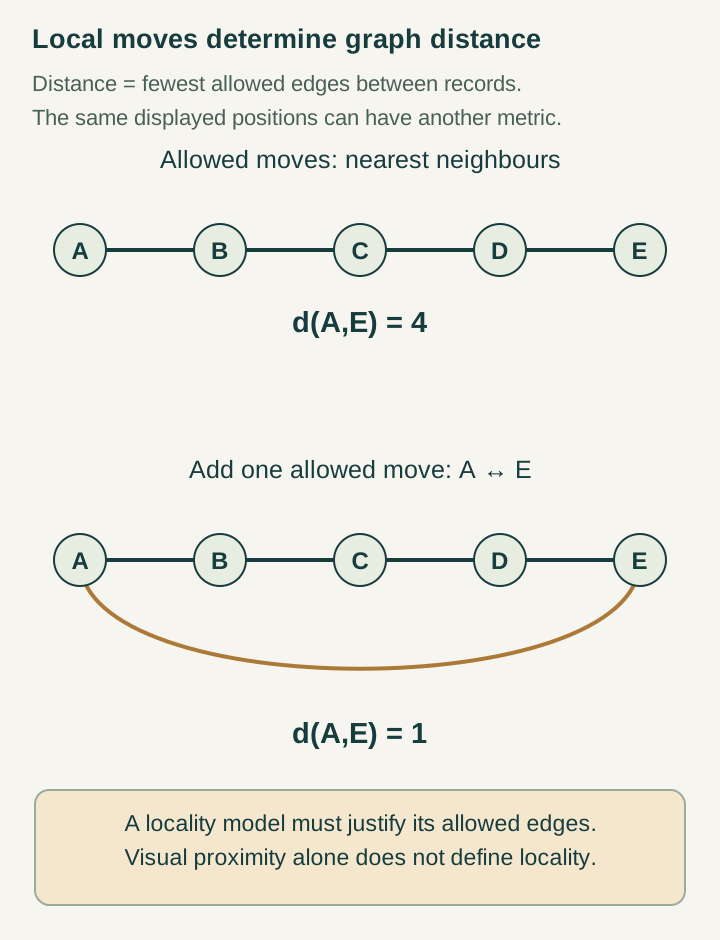
Open the full-size diagram →
Why a local update preserves that neighborhood
Give each site local registers and distinct edge ports. Let one completed episode consist of an on-site operation followed by a single layer exchanging only designated neighboring ports. The port pairs are disjoint, so the edge layer does not conceal additional sequential travel. An observable initially supported on X can gain support only on neighbors of X during one episode.
Induction gives support after k episodes inside the graph neighborhood B(X,k). Applying the same one-step argument to the previous support proves each induction step. This is an exact circuit result with a declared interaction architecture. A distant arbitrary swap or a controller carrying unknown state between nonadjacent sites would change that architecture and invalidate the bound. The source mechanism must account for such channels before claiming physical locality.
How a support bound becomes a causal speed
Assign an independently calibrated edge length ℓ and an episode duration ΔT. The graph bound supplies propagation slope at most ℓ/ΔT. If ℓ=2 length units and ΔT=3 clock units, five episodes permit at most ten length units in fifteen clock units, again giving 2/3. Counting a completed episode as one tick is insufficient unless a material clock establishes its duration.
More generally, assume each completed operation has positive delay Θ and displacement satisfying ‖Δx‖≤c⋆Θ. Concatenation preserves this cone: the triangle inequality gives ‖ΣΔx‖≤Σ‖Δx‖≤c⋆ΣΘ. This is a useful exact compositional theorem. Identifying its slope with a universal physical light speed requires the same calibrated bound to govern the relevant matter and signals, rather than only a selected circuit or propagation band.
From a cone symmetry to physical relativity
Once an interval T²−x² with T=ct is supplied, the boost T′=γ(T−βx), x′=γ(x−βT) preserves it. For β=3/5, γ=5/4. The event separation T=5,x=3 becomes T′=4,x′=0, preserving sixteen. Split-complex multiplication is one exact way to express this hyperbolic transformation.
The model must still show that real clocks, rods and moving apparatus realize those transformations. A geometrical automorphism is not automatically an available observer. A sufficient group-theoretic condition is physical realization of all spatial rotations plus transitivity on future unit timelike directions within the proper orthochronous Lorentz group. Any desired boost can then be matched on the rest direction by a physical transformation; their difference fixes rest and is a physical rotation. The remaining challenge is deriving those operational conditions.
Why a programmed lattice is an important first step
The finite archive proves that a common update can support local records. Explaining why that structure forms and persists is stronger. A source may use a structured initial register, a restricted family of operations or a repair process. Each possibility must disclose its preparation and memory resources. Statistical rarity results for unstructured random operation tables do not rule out all these mechanisms, but they show why selection cannot simply be assumed.
Perturb the neighborhood tables and inspect shortest unintended paths as well as the fraction of local errors. One shortcut can change a large-distance route even if almost every edge remains correct. Then perturb the dynamics and bound influence leakage. These tests turn emergent locality into a quantitative stability problem. The six nested inner roles can organize formation and verification, while outer completion must expose a usable archive with its actual preparation duration.
Serial generation must include the cost of its schedule
An inner process may visit records one at a time while a completed episode displays a whole neighborhood. The corresponding causal bound depends on when the displayed data become available to other operations. Suppose a source updates a chain of five registers from left to right. If each later register reads the value just written into its predecessor, a disturbance can travel from the first register to the fifth during one sweep. Calling the entire sweep one local step conceals four sequential transmissions.
By contrast, an update that reads only a retained previous layer and writes a separate next layer propagates at most one edge per completed step. The two procedures use the same drawn chain and the same local update formula, yet their schedules give different support bounds. A physical model must account for the second register bank or equivalent protected memory needed by the latter implementation. The timing and retention mechanism carry information that an adjacency diagram alone omits.
This is a useful role for nested generation: higher-level completion can prevent unfinished lower-level results from acting as completed inputs. The gate must be part of the update, and its own communication channels must be included. An observer should not be granted access to a private scheduling register unless that access is an admitted physical measurement. Such access could reveal a preferred order that is absent from the completed relational description.
Compare geometry and clocks across more than one preparation
Suppose one preparation yields edge length two and episode duration three, while a second yields edge length four and duration six. Their upper propagation slopes agree at two-thirds. If a third preparation changes only duration to four while retaining edge length two, its slope is one-half. A universal coefficient requires a reason to exclude that independent change or a different account of the measured quantities.
The useful source question is whether one conserved relation or interaction forces length and clock response to change together. The quantities should be measured separately before their ratio is formed. Calibrating the clock from the desired propagation slope would make the agreement automatic. A fixed family of preparations, together with independently constructed clocks and rulers, can expose which source parameters remain free.
This comparison also distinguishes unit conventions from physical agreement. Changing the chosen length unit rescales all expressed speeds consistently. Changing one clock coupling while keeping the common reference procedure fixed changes a physical comparison that the source model must predict.
A common graph need not give every field the same speed
Consider two signal registers at every site of a chain. During each calibrated episode, species A advances one edge, while species B advances only on alternating episodes. Both use the same adjacency and the same outer clock; their maximal average speeds are ℓ/ΔT and ℓ/(2ΔT). The difference is a supplied update rule. Source unity does not remove it simply because both rules execute on one controller.
There may nevertheless be a shared upper bound c⋆=ℓ/ΔT. A common speed limit is weaker than the assertion that every massless excitation has a dispersion relation with that slope. Slow matter is compatible with a shared causal cone, but identifying a particular field with light needs a dynamical reason that its relevant signal propagation saturates the selected cone. A group velocity extracted from one band and a strict support front are also different observables.
The constructive comparison keeps the graph, clock apparatus and length calibration fixed while changing permitted field preparations. Compute front support and band dispersion separately. If a source symmetry or common coupling forces their limiting coefficients to agree in a stated regime, that is an identifiable advance. If two freely adjustable coefficients survive, the model reveals a specific coupling or calibration problem to solve.
Quantify the effect of a small nonlocal channel
An exact circuit locality theorem excludes every unauthorized edge. An approximate realization needs an error estimate. Suppose U is the intended unitary step and V is the realized step, with operator-norm difference at most ε. Both are unitary. Expanding Vᵏ−Uᵏ as a telescoping sum gives a norm bound kε: each term contains one factor V−U surrounded by norm-one factors. No assumption that the two steps commute is needed.
The second estimate follows by adding and subtracting V†ᵏOUᵏ and using the first bound twice. It controls how much a bounded observable can differ from the exactly local model after k steps. If the ideal Heisenberg observable commutes with a distant bounded probe B, the realized commutator is at most 4kε‖O‖‖B‖. The estimate is useful for short controlled runs, although it becomes loose as kε grows.
A long-time theory needs a stronger statement, perhaps from the structure of the unwanted terms or from a repair mechanism with its own bounded influence. This calculation demonstrates the form a checkable stability claim should take: name a norm, a preparation class, an observation time and a tolerated error. A small fraction of incorrect edges is not an adequate substitute because a single shortcut can alter a macroscopic distance.
These diagnostics connect the geometric and physical parts of SMM/DTT without presuming their final answer. They ask whether six nested dependencies, retained local ports and the completion interface can enforce a common causal organization under finite imperfections. The meaningful result is a relation between operationally defined quantities that survives declared perturbations, not merely an exact symmetry of an ideal diagram.
What a successful source reconstruction would deliver
The strongest result would generate adjacency, metric comparisons, material clocks and propagation with one fixed interaction law. It would show that a private generative schedule does not furnish an extra public simultaneity detector. Across changing preparations, moving clocks would retain the derived calibration and matter would share the same causal structure.
A Lorentzian metric is an important kinematic output; gravitational field equations require additional dynamics relating geometry to matter. A local circuit bound likewise does not establish Einstein’s equations. These are concrete next targets rather than interchangeable slogans. The constructive answer is that locality and relativity can be approached through exact operational steps, and SMM/DTT gains explanatory strength wherever one source principle forces two of those steps to agree.
Continue with the articles
- Programmed geometry and spontaneous selection
A programmed serial source can prepare a periodic lattice and reproduce its local neighborhoods exactly. This establishes feasibility while leaving spontaneous selection, dimension choice, and persistent growth as separate tasks.
- Generating a neighborhood and preserving local transport
A generated graph predicts local influence only when later operations respect its edges and retained ports. Guarded transport supplies a finite-update support bound while exposing runtime and controller-memory requirements.
- From a cone inequality to a Lorentzian metric
A positive horizontal metric and a nonzero temporal one-form define a Lorentzian metric with one negative direction. The signature proof leaves clock integrability, observer equivalence, and gravitational dynamics distinct.
- Limiting speed as update scale times projection rate
The limiting-speed factorization c=κρ combines a spatial update scale with a phase-to-clock rate. It is dimensionally consistent but does not independently select either microscopic factor or a numerical speed.
- Why light must share the same cone
Light follows the constructed null cone if its electromagnetic constitutive law uses the same metric. A countermodel with another field speed shows why common geometry does not alone establish universal propagation.
- When geometric symmetries become physical boosts
A geometry can admit Lorentz transformations that its material observers cannot realize. The frame-richness argument identifies the extra reachability and clock-calibration conditions needed to turn geometric automorphisms into physical boosts.
- What Lorentzian reconstruction leaves open
Lorentzian reconstruction provides a conditional account of observer geometry without determining matter, coupling constants or gravitational dynamics. This guide identifies the source-level results still needed to connect clocks, propagation and curvature.
Develop the argument
Questions to take further
- Does a serial implementation preserve the support bound when its scheduling memory is included?
- Which source restriction forces the relevant field and physical clocks to share one causal coefficient?
A concrete next step
Audit a generated causal neighborhood
Specify all local registers, scheduling memory and read/write permissions; calibrate duration and compare two matter channels.
What to share
An exact support proof, a finite perturbation bound and a table of independently measured front and band velocities.
I welcome collaboration with experts in physics, mathematics and philosophy. Get in touch with a question or proposal.